评分卡模型
为了设计一个专家评分模型,可以采用以下步骤:
- 确定评分指标:首先,确定评分模型的目标和评估标准。根据具体的领域或任务,确定需要考虑的关键指标,例如准确性、可靠性、创新性等。
- 收集专家数据:收集一组专家的评分数据,这些专家应该具有相关领域的专业知识和经验。可以通过面对面的访谈、问卷调查或在线平台来收集数据。
- 构建评分模型:选择合适的机器学习算法或统计模型来构建评分模型。常见的方法包括回归分析、决策树、支持向量机等。根据数据的特点和评分指标的要求,选择最合适的模型。
- 特征工程:根据收集到的专家数据,将评分指标转化为特征。这可能包括对数据进行清洗、归一化或转换等预处理步骤。还可以考虑添加一些领域相关的特征,以提高模型的性能。
- 模型训练和验证:将专家数据分为训练集和验证集,使用训练集对模型进行训练,并使用验证集对模型进行验证和调优。可以使用交叉验证等技术来评估模型的性能。
- 模型评估和解释:评估模型的性能,包括准确性、召回率、精确度等指标。同时,对模型的结果进行解释,以便专家能够理解评分的依据和原因。
- 持续改进:根据评估结果和专家的反馈,对模型进行改进和优化。可以通过增加更多的专家数据、调整模型参数或改进特征工程等方式来提高模型的性能。
评分模型的设计和实施是一个迭代的过程,需要不断地与专家进行交流和改进。同时,模型的性能也受到数据质量和领域知识的影响,因此在设计评分模型时需要综合考虑多个因素。
信用评分卡建模过程
信用评分卡是一个通过个人数据对其还款能力、还款意愿进行定量评估的系统。
建模流程
信用风险评级模型的主要开发流程如下: (1) 获取数据,包括申请贷款客户的数据。数据包括客户各个维度,包括年龄,性别,收入,职业,家人数量,住房情况,消费情况,债务等等。 (2) 数据预处理,主要工作包括数据清洗、缺失值处理、异常值处理、数据类型转换等等。我们需要把原始数据层层转化为可建模数据。 (3) EDA探索性数据分析和描述性统计,包括统计总体数据量大小,好坏客户占比,数据类型有哪些,变量缺失率,变量频率分析直方图可视化,箱形图可视化,变量相关性可视化等。 (4) 变量选择,通过统计学和机器学习的方法,筛选出对违约状态影响最显著的变量。常见变量选择方法很多,包括iv,feature importance,方差等等 。另外缺失率太高的变量也建议删除。无业务解释性变量且没有价值变量也建议删除。 (5) 模型开发,评分卡建模主要难点是woe分箱,分数拉伸,变量系数计算。其中woe分箱是评分卡中难点中难点,需要丰富统计学知识和业务经验。目前分箱算法多达50多种,没有统一金标准,一般是先机器自动分箱,然后再手动调整分箱,最后反复测试模型最后性能,择优选取最优分箱算法。 (6) 模型验证,核实模型的区分能力、预测能力、稳定性、排序能力等等,并形成模型评估报告,得出模型是否可以使用的结论。模型验证不是一次性完成,而是当建模后,模型上线前,模型上线后定期验证。模型开发和维护是一个循环周期,不是一次完成。 (7) 信用评分卡,根据逻辑回归的变量系数和WOE值来生成评分卡。评分卡方便业务解释,已使用几十年,非常稳定,深受金融行业喜爱。其方法就是将Logistic模型概率分转换为300-900分的标准评分的形式。 (8) 建立评分卡模型系统,根据信用评分卡方法,建立计算机自动信用化评分系统。美国传统产品FICO有类似功能,FICO底层语言是Java。目前流行Java,python或R多种语言构建评分卡自动化模型系统。
(9)模型监控,着时间推移,模型区分能力,例如ks,auc会逐步下降,模型稳定性也会发生偏移。我们需要专业模型监控团队,当监控到模型区分能力下降显著或模型稳定性发生较大偏移时,我们需要重新开发模型,迭代模型。如图:

导入数据
该模型数据集来源于kaggle网站的Give Me Some Credit,数据包括了25万条个人财务情况的样本数据,通过对于该数据集的学习,构建一个信用卡评分模型,以期望对新用户预测其违约风险。
输出数据的基本信息
# 导入库
import pandas as pd
import numpy as np
import matplotlib.pyplot as plt
import matplotlib
import toad as td

def card_train():
    # 导入训练集
	train = pd.read_csv('./data/cs-training.csv')

    # 设置matplotlib正常显示中文和负号
    matplotlib.rcParams['font.sans-serif'] = ['SimHei']  # 用黑体显示中文
    matplotlib.rcParams['axes.unicode_minus'] = False    # 正常显示负号

    print("输出样本数据的相关信息概览")
    train.info()
样本数据输出结果
样本数据的相关信息概览
-----------------------------------------------------------------------------------------
<class 'pandas.core.frame.DataFrame'>
RangeIndex: 150000 entries, 0 to 149999
Data columns (total 12 columns):
 #   Column                                Non-Null Count   Dtype
---  ------                                --------------   -----
 0   ID                                    150000 non-null  int64
 1   SeriousDlqin2yrs                      150000 non-null  int64
 2   RevolvingUtilizationOfUnsecuredLines  150000 non-null  float64
 3   age                                   150000 non-null  int64
 4   NumberOfTime30-59DaysPastDueNotWorse  150000 non-null  int64
 5   DebtRatio                             150000 non-null  float64
 6   MonthlyIncome                         120269 non-null  float64
 7   NumberOfOpenCreditLinesAndLoans       150000 non-null  int64
 8   NumberOfTimes90DaysLate               150000 non-null  int64
 9   NumberRealEstateLoansOrLines          150000 non-null  int64
 10  NumberOfTime60-89DaysPastDueNotWorse  150000 non-null  int64
 11  NumberOfDependents                    146076 non-null  float64
dtypes: float64(4), int64(8)
memory usage: 13.7 MB
通过样本输出数据可以看到样本数有15万条,特征变量有12个,具体各变量的含义如下
| 标号 | 变量 | 变量说明 |
|---|---|---|
| x0 | ID | 编号 |
| x1 | SeriousDlqin2yrs | 好/坏客户 |
| x2 | RevolvingUtilizationOfUnsecuredLines | 无担保放款的循环利用 |
| x3 | age | 年龄 |
| x4 | NumberOfTime30-59DaysPastDueNotWorse | 30-59天逾期次数(不严重) |
| x5 | DebtRatio | 负债比例 |
| x6 | MonthlyIncome | 月收入 |
| x7 | NumberOfOpenCreditLinesAndLoans | 信贷和贷款数量 |
| x8 | NumberOfTimes90DaysLate | 90天逾期次数 |
| x9 | NumberRealEstateLoansOrLines | 不动产贷款或额度数量 |
| x10 | NumberOfTime60-89DaysPastDueNotWorse | 60-89天逾期次数 |
| x11 | NumberOfDependents | 家属数量(人数) |
样本前5条数据,为便于展示,表头使用中文显示且只展示部分列
| 好/坏客户 | 无担保放款 | 年龄 | 负债比例 | 月收入 | 贷款数量 | 90天逾期次数 | 家属数量 |
|---|---|---|---|---|---|---|---|
| 1 | 0.766127 | 45 | 0.802982 | 9120.0 | 13 | 0 | 2.0 |
| 0 | 0.957151 | 40 | 0.121876 | 2600.0 | 4 | 0 | 1.0 |
| 0 | 0.658180 | 38 | 0.085113 | 3042.0 | 2 | 1 | 0.0 |
| 0 | 0.233810 | 30 | 0.036050 | 3300.0 | 5 | 0 | 0.0 |
| 0 | 0.907239 | 49 | 0.024926 | 63588.0 | 7 | 0 | 0.0 |
数据集的EDA数据
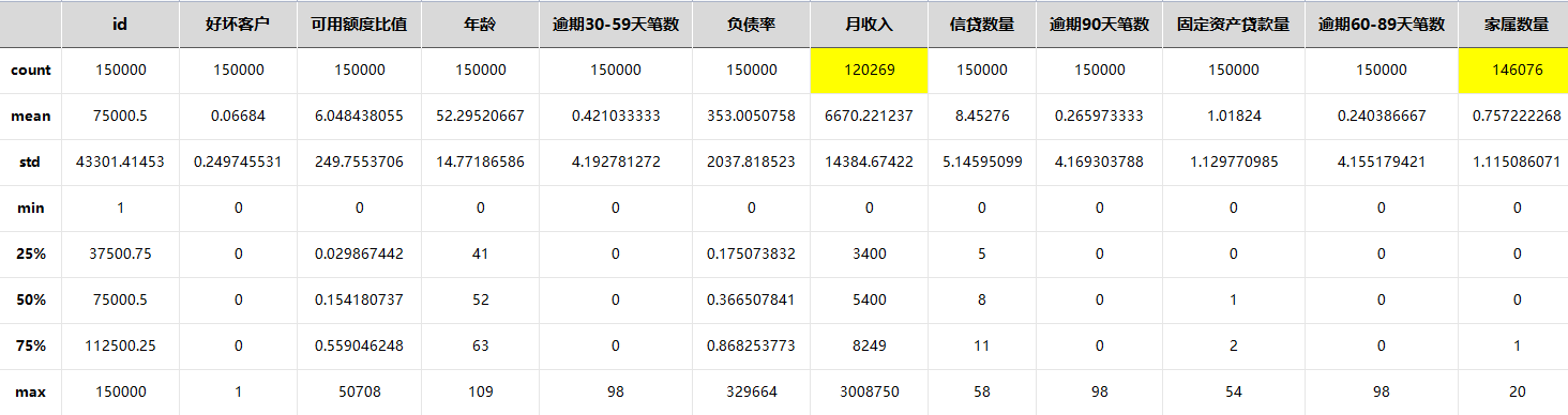
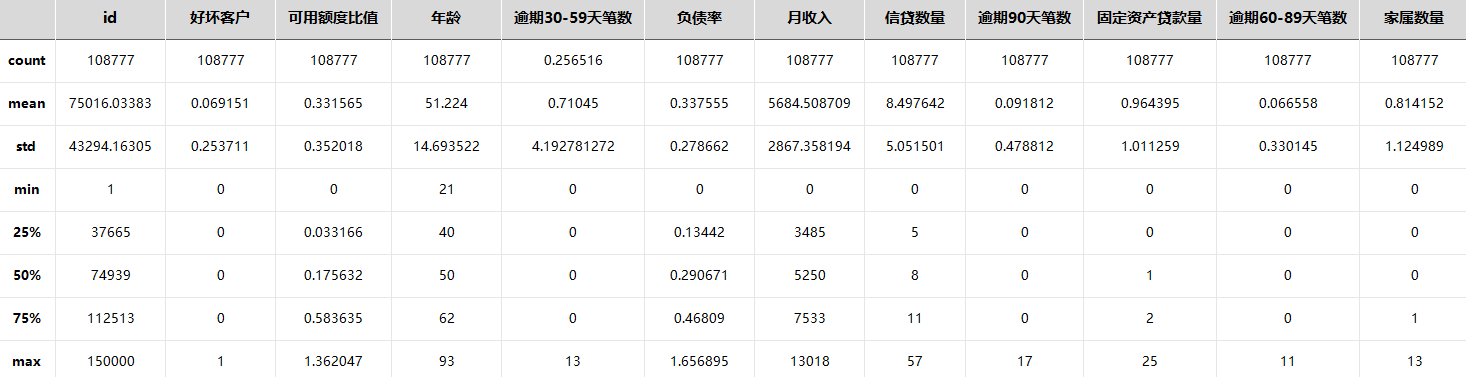
上述EDA表发现变量月收入和家庭数量的样本数小于15w,两个变量存在缺失值。
月收入缺失比:19.82%
家属数量缺失比:2.62%
缺失值处理
缺失值的类型:完全随机缺失,随机缺失,非随机缺失 处理方法: 1、删除含有缺失值的个案 2、可能值插补缺失值 (1)均值插补 (2)利用同类均值插补。 (3)极大似然估计(Max Likelihood ,ML) (4)多重插补(Multiple Imputation,MI)
月收入的缺失比较大,应该进行缺失值的估计插补,此处采用均值插补方法,月收入变量数据为定距型,采用该变量的均值进行填补。
家属数量的缺失比较低,可以直接删除有缺失的样本。
# 用均值填补月收入缺失值
train['MonthlyIncome'] = train['MonthlyIncome'].fillna(train['MonthlyIncome'].mean())

# 删除存在缺失值的样本(删除家属数量缺失数据)
train = train.dropna()
train.info()
缺失值处理后的样本数据
缺失值处理后的样本数据的相关信息概览
-----------------------------------------------------------------------------------------
<class 'pandas.core.frame.DataFrame'>
RangeIndex: 150000 entries, 0 to 149999
Data columns (total 12 columns):
 #   Column                                Non-Null Count   Dtype
---  ------                                --------------   -----
 0   ID                                    146076 non-null  int64
 1   SeriousDlqin2yrs                      146076 non-null  int64
 2   RevolvingUtilizationOfUnsecuredLines  146076 non-null  float64
 3   age                                   146076 non-null  int64
 4   NumberOfTime30-59DaysPastDueNotWorse  146076 non-null  int64
 5   DebtRatio                             146076 non-null  float64
 6   MonthlyIncome                         146076 non-null  float64
 7   NumberOfOpenCreditLinesAndLoans       146076 non-null  int64
 8   NumberOfTimes90DaysLate               146076 non-null  int64
 9   NumberRealEstateLoansOrLines          146076 non-null  int64
 10  NumberOfTime60-89DaysPastDueNotWorse  146076 non-null  int64
 11  NumberOfDependents                    146076 non-null  float64
dtypes: float64(4), int64(8)
memory usage: 13.7 MB
异常值处理
异常值即离群点,一般大于3倍标准差外的数值为异常值,可以采用箱线图判断异常值。
通过画出样本数据的箱线图查看异常数据
# 画箱线图,采用组合图的方式
fig = plt.figure(figsize=(15, 10))
a = fig.add_subplot(3, 2, 1)
b = fig.add_subplot(3, 2, 2)
c = fig.add_subplot(3, 2, 3)
d = fig.add_subplot(3, 2, 4)
e = fig.add_subplot(3, 2, 5)
f = fig.add_subplot(3, 2, 6)

a.boxplot(train['RevolvingUtilizationOfUnsecuredLines'], labels=("可用额度",))
b.boxplot([train['age'], train['SeriousDlqin2yrs']], labels=("年龄","好坏客户",))
c.boxplot([
    train['NumberOfTime30-59DaysPastDueNotWorse'],
    train['NumberOfTime60-89DaysPastDueNotWorse'],
    train['NumberOfTimes90DaysLate']],
    labels=("逾期30-59天","逾期60-90天","逾期90天以上",))
d.boxplot([
    train['NumberOfOpenCreditLinesAndLoans'],
    train['NumberRealEstateLoansOrLines'],
    train['NumberOfDependents']],
    labels=("信贷","固定资产贷","家属",))
e.boxplot(train['MonthlyIncome'], labels=("月收入",))
f.boxplot(train['DebtRatio'], labels=("负债率",))
plt.suptitle("箱线图", fontsize=22)
plt.show()
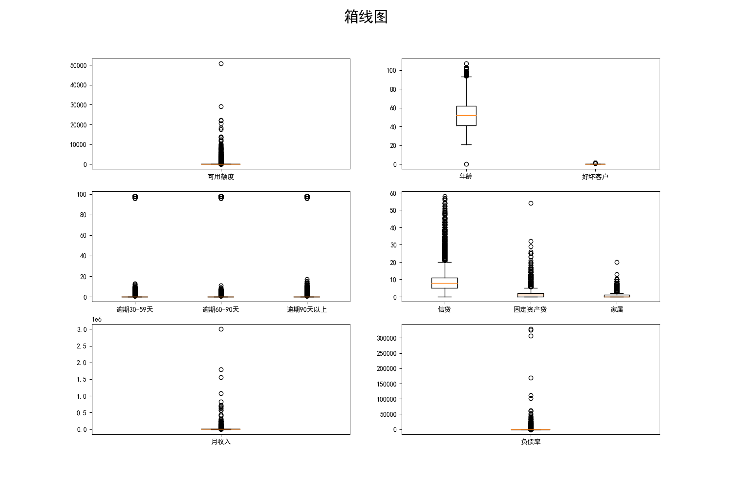
从图中可以看出,处在箱线图上下边缘之外的为异常值。用公式去除异常值,计算第一和第三四分位数(Q1、Q3),异常值是位于四分位数范围之外的数据点x i:

使用四分位数乘数值k=1.5,范围限制是典型的上下晶须的盒子图。计算出来的正是箱线图的上下限。
# 去可用额度比值、年龄、负债率、月收入的除异常值
for k in [2, 3, 5, 6]:  # 遍历列
    q1 = train.iloc[:, k].quantile(0.25)  # 计算上四分位数
    q3 = train.iloc[:, k].quantile(0.75)  # 计算下四分位数
    iqr = q3 - q1
    low = q1 - 1.5 * iqr
    up = q3 + 1.5 * iqr
    if k == 2:
        train1 = train
        # 保留正常值范围
        train1 = train1[(train1.iloc[:, k] > low) & (train1.iloc[:, k] < up)]
        train = train1
        train.info()
        train.iloc[:, [2, 3, 5, 6]].boxplot(figsize=(15, 10))
        plt.suptitle("箱线图", fontsize=22)
        plt.show()
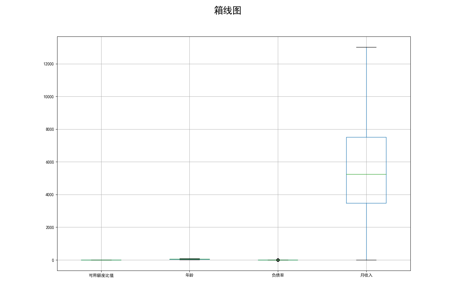
去掉异常值后,通过观察箱线图,发现这四个变量已经不存在异常值,再依次去掉其他变量的异常值。
异常值处理后的样本数据
异常值处理后的样本数据的相关信息概览
-----------------------------------------------------------------------------------------
<class 'pandas.core.frame.DataFrame'>
RangeIndex: 150000 entries, 0 to 149999
Data columns (total 12 columns):
 #   Column                                Non-Null Count   Dtype
---  ------                                --------------   -----
 0   ID                                    108991 non-null  int64
 1   SeriousDlqin2yrs                      108991 non-null  int64
 2   RevolvingUtilizationOfUnsecuredLines  108991 non-null  float64
 3   age                                   108991 non-null  int64
 4   NumberOfTime30-59DaysPastDueNotWorse  108991 non-null  int64
 5   DebtRatio                             108991 non-null  float64
 6   MonthlyIncome                         108991 non-null  float64
 7   NumberOfOpenCreditLinesAndLoans       108991 non-null  int64
 8   NumberOfTimes90DaysLate               108991 non-null  int64
 9   NumberRealEstateLoansOrLines          108991 non-null  int64
 10  NumberOfTime60-89DaysPastDueNotWorse  108991 non-null  int64
 11  NumberOfDependents                    108991 non-null  float64
dtypes: float64(4), int64(8)
memory usage: 10.8 MB
# 分别去掉各变量的异常值
train = train[train['NumberOfTime30-59DaysPastDueNotWorse'] < 80]
train = train[train['NumberOfTime60-89DaysPastDueNotWorse'] < 80]
train = train[train['NumberOfTimes90DaysLate'] < 80]
train = train[train['NumberRealEstateLoansOrLines'] < 50]
train = train[train['NumberOfDependents'] < 15]

# 去掉重复样本
train.drop_duplicates(inplace=True)
print(train.describe())
数据集处理异常后的EDA数据
探索性分析
判断各个特征变量是否满足统计基本假设,即连续型变量应该满足近似正态分布的假设。分别绘制直方图进行分析。
# 探索性分析( EDA ) 画出直方图
train.hist(figsize=(20, 15))
plt.subplots_adjust(hspace=0.5)
plt.suptitle("直方图", fontsize=22)
plt.show()
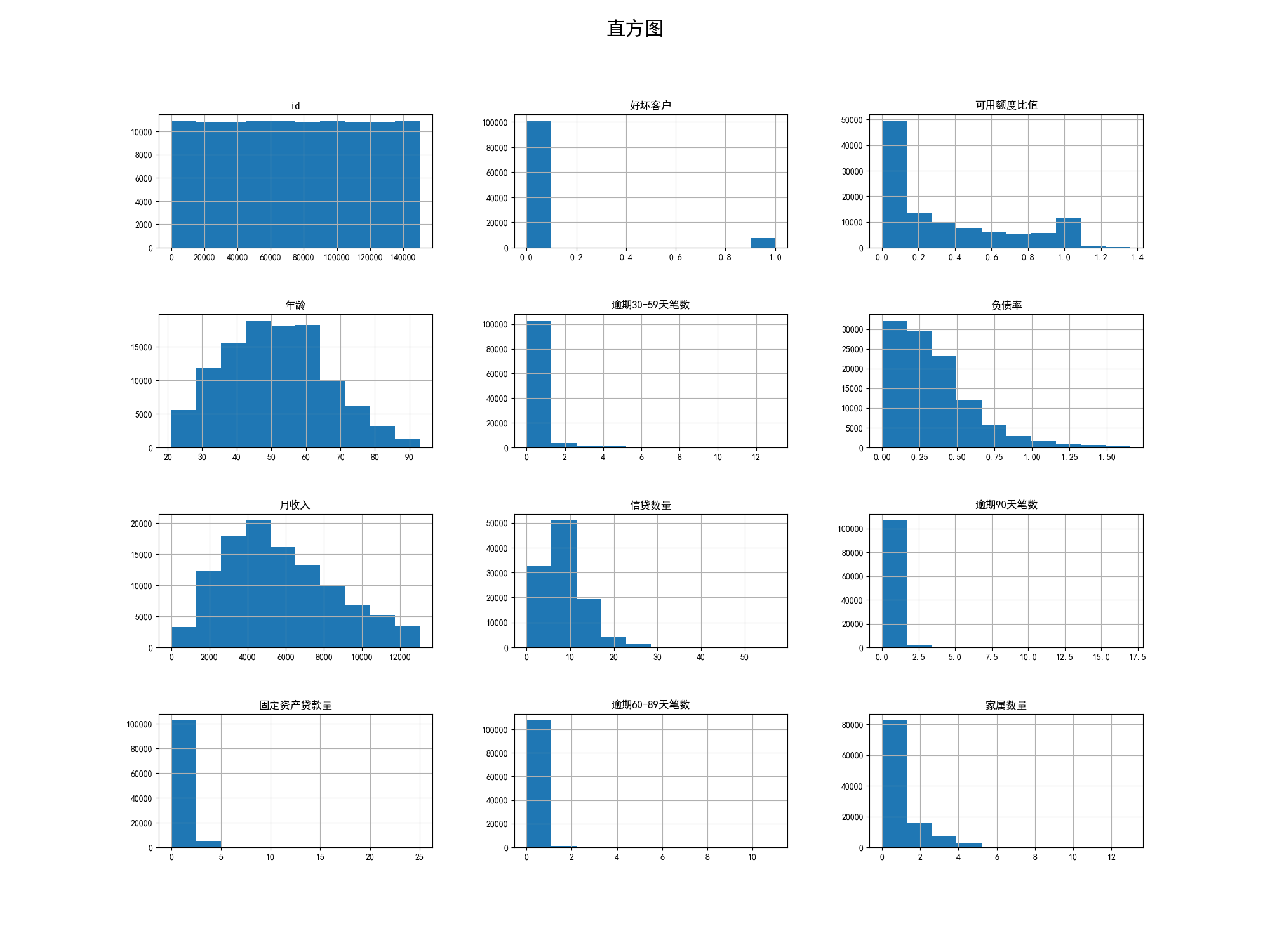
直方图表明年龄和月收入近似服从正态分布,符合一般统计假设,可用额度比值和负债率的分布也较为均匀。
变量选择
为了预测新样本为好/坏客户,训练集有标签标记,是有监督学习,一个二分类问题,可以采用logistic回归进行分类,为了训练处分类器,要进行自变量的选择,可以采用IV(Information Value 信息量)来判断选择,IV可以衡量自变量的预测能力,IV计算要以WOE(证据权重)为基础,WOE是对原始自变量的一种编码形式,要对一个变量进行WOE编码,需要首先把这个变量进行分组处理(也叫离散化、分箱等等),因此,对项目中的连续型变量进行分箱处理。
分箱处理
变量分箱的方法有等距分段、等深分段、最优分段,其中等距分段(Equval length intervals)是指分段的区间是一致的,比如年龄以十年作为一个分段;等深分段(Equal frequency intervals)是先确定分段数量,然后令每个分段中数据数量大致相等;最优分段(Optimal Binning)又叫监督离散化(supervised discretizaion),使用递归划分(Recursive Partitioning)将连续变量分为分段,背后是一种基于条件推断查找较佳分组的算法。
利用所定义的函数依次对连续型变量进行最优分段分箱处理,得到各个分箱数据和woe值。WOE的定义如下:
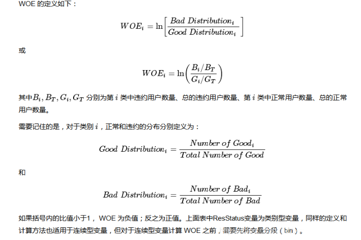
从上式中可以发现,WOEi 为第 i 类中违约与正常的比率与整个样本中违约与正常比率的比值的对数。因此,其目的是衡量第 i 类对违约与正常的比率的影响程度。|WOEi| 越大,说明此类别更能区分违约与正常用户,|WOEi| 越小,此类别区分违约与正常不明显。
通常,对连续型变量进行分箱计算WOE之后,其各个分箱的WOE值应该呈现一个单调趋势。当然,有时连续性变量的WOE也有可能呈现一个U型趋势(比如在上面前言中评分卡的变量Age)。不管如何,首先都要从业务上能给出一个合理的解释,否则,这个变量很可能没法放到我们最后创建的评分卡中。
# 去掉重复样本
x1=op(train['SeriousDlqin2yrs'],train['age'])
x2=op(train['SeriousDlqin2yrs'],train['DebtRatio'])
x3=op(train['SeriousDlqin2yrs'],train['MonthlyIncome'])

# 最优分段分箱(年龄)
print(x1)
# 最优分段分箱(负债率)
print(x2)
# 最优分段分箱(月收入)
print(x3)

x1=funqcut(train['SeriousDlqin2yrs'],
           train['RevolvingUtilizationOfUnsecuredLines'],5).reset_index()
x2=funqcut(train['SeriousDlqin2yrs'],train['age'],12).reset_index()
x4=funqcut(train['SeriousDlqin2yrs'],train['DebtRatio'],4).reset_index()
x5=funqcut(train['SeriousDlqin2yrs'],train['MonthlyIncome'],5).reset_index()
x6=funqcut(train['SeriousDlqin2yrs'],
           train['NumberOfOpenCreditLinesAndLoans'],6).reset_index()

# 深度分段分箱(可用额度比值)
print(x1)
# 深度分段分箱(年龄)
print(x2)
# 深度分段分箱(负债率)
print(x4)
# 深度分段分箱(月收入)
print(x5)
# 深度分段分箱(信贷数量)
print(x6)

x3 = funqcut(train['SeriousDlqin2yrs'],
             train['NumberOfTime30-59DaysPastDueNotWorse'], 5).reset_index()
x9 = funqcut(train['SeriousDlqin2yrs'],
             train['NumberOfTime60-89DaysPastDueNotWorse'], 5).reset_index()
x7 = funqcut(train['SeriousDlqin2yrs'],
             train['NumberOfTimes90DaysLate'], 5).reset_index()
x8 = funqcut(train['SeriousDlqin2yrs'],
             train['NumberRealEstateLoansOrLines'], 5).reset_index()
x10= funqcut(train['SeriousDlqin2yrs'],
             train['NumberOfDependents'], 5).reset_index()

# 深度分段分箱(逾期30-59天笔数)
print(x3)
# 深度分段分箱(逾期60-89天笔数)
print(x9)
# 深度分段分箱(逾期90天笔数)
print(x7)
# 深度分段分箱(固定资产贷款量)
print(x8)
# 深度分段分箱(家属数量)
print(x10)
输出结果如下:
最优分段分箱(年龄)
-----------------------------------------------------------------------------------------
    min  max  sum  total      rate       woe
0    21   30  932   8599  0.108385 -4.707158
1    31   34  709   7033  0.100810 -4.788062
2    35   38  729   7766  0.093871 -4.867074
3    39   41  653   7120  0.091713 -4.892700
4    42   44  608   7390  0.082273 -5.011662
..  ...  ...  ...    ...       ...       ...
10   59   61  363   6792  0.053445 -5.473981
11   62   64  289   6771  0.042682 -5.710168
12   65   68  199   6450  0.030853 -6.047002
13   69   75  208   7583  0.027430 -6.168123
14   76   93  143   6660  0.021471 -6.419135

[15 rows x 6 columns]

最优分段分箱(负债率)
-----------------------------------------------------------------------------------------
        min       max   sum  total      rate       woe
0  0.000000  0.134420  1571  27195  0.057768 -5.391627
1  0.134425  0.290671  1607  27194  0.059094 -5.367525
2  0.290674  0.468090  1677  27194  0.061668 -5.322148
3  0.468097  1.656895  2667  27194  0.098073 -4.818630

最优分段分箱(月收入)
-----------------------------------------------------------------------------------------
      min           max   sum  total      rate       woe
0     0.0   2833.000000  1647  18150  0.090744 -4.904397
1  2834.0   4000.000000  1573  18312  0.085900 -4.964567
2  4001.0   5250.000000  1371  18037  0.076010 -5.097640
3  5251.0   6670.221237  1200  18636  0.064392 -5.276026
4  6671.0   8740.000000   922  17512  0.052650 -5.489820
5  8741.0  13018.000000   809  18130  0.044622 -5.663686

深度分段分箱(可用额度比值)
-----------------------------------------------------------------------------------------
可用额度比值  			坏客户数  好客户数       woe        iv
0     (0.999, 21756.2]   456  21300 		-1.244160  	0.186298
1   (21756.2, 43511.4]   404  21351 		-1.367629  	0.214929
2   (43511.4, 65266.6]   726  21029 		-0.766298  	0.085187
3   (65266.6, 87021.8]  1659  20096  		0.105504  	0.002330
4  (87021.8, 108777.0]  4277  17479  		1.192062  	0.472027

深度分段分箱(年龄)
-----------------------------------------------------------------------------------------
年龄  									坏客户数  好客户数       woe        iv
0        (0.999, 9065.667]   982  		8083  0.491883  	0.024949
1    (9065.667, 18130.333]   908  		8157  0.404423  	0.016239
2     (18130.333, 27195.0]   818 		  8247  0.289068  	0.007891
3     (27195.0, 36259.667]   797  		8267  0.260638  	0.006336
4   (36259.667, 45324.333]   724  		8341  0.155663  	0.002160
..                     ...   ...   		...       ...       ...
7   (63453.667, 72518.333]   561  		8504 -0.118761  	0.001117
8     (72518.333, 81583.0]   480  		8585 -0.284176  	0.005960
9     (81583.0, 90647.667]   360  		8704 -0.585624  	0.022313
10  (90647.667, 99712.333]   254  		8811 -0.946612  	0.050407
11   (99712.333, 108777.0]   210  		8855 -1.141820  	0.067978

[12 rows x 5 columns]

深度分段分箱(负债率)
-----------------------------------------------------------------------------------------
负债率  				 坏客户数   好客户数       woe        iv
0     (0.999, 27195.0]  1571  	25624 	-0.192007  	0.008489
1   (27195.0, 54389.0]  1607 	25587 	-0.167905  	0.006558
2   (54389.0, 81583.0]  1677  	25517 	-0.122528  	0.003561
3  (81583.0, 108777.0]  2667  	24527  	0.380990  	0.042797

深度分段分箱(月收入)
-----------------------------------------------------------------------------------------
月收入  				坏客户数   好客户数     woe            iv
0     (0.999, 21756.2]  1987  	19769  0.302321  2.083557e-02
1   (21756.2, 43511.4]  1802  	19953  0.195328  8.302796e-03
2   (43511.4, 65266.6]  1503  	20252 -0.000980  1.921583e-07
3   (65266.6, 87021.8]  1231  	20524 -0.213958  8.353539e-03
4  (87021.8, 108777.0]   999  	20757 -0.434074  3.133444e-02

深度分段分箱(信贷数量)
-----------------------------------------------------------------------------------------
信贷数量  			     坏客户数   	好客户数       woe        iv
0      (0.999, 18130.333]  1800  	16330  		0.394593  	0.030787
1  (18130.333, 36259.667]  1222  	16907 		-0.027429  	0.000124
2    (36259.667, 54389.0]  1027  	17103 		-0.212802  	0.006890
3    (54389.0, 72518.333]  1077  	17052 		-0.162278  	0.004094
4  (72518.333, 90647.667]  1147  	16982 		-0.095194  	0.001450
5   (90647.667, 108777.0]  1249  	16881 		-0.004035  	0.000003

深度分段分箱(逾期30-59天笔数)
-----------------------------------------------------------------------------------------
逾期30-59天笔数  			坏客户数   好客户数       woe        iv
0     (0.999, 21756.2]   	943  	20813 	-0.494457  	0.039648
1   (21756.2, 43511.4]   	932  	20823 	-0.506671  	0.041418
2   (43511.4, 65266.6]   	879  	20876 	-0.567761  	0.050710
3   (65266.6, 87021.8]   	930  	20825 	-0.508915  	0.041747
4  (87021.8, 108777.0]  	3838  	17918  	1.058956  	0.352926

深度分段分箱(逾期60-89天笔数)
-----------------------------------------------------------------------------------------
逾期60-89天笔数  				坏客户数   	 好客户数         woe        iv
0     (0.999, 21756.2]  		1128 		20628 	-0.306393  0.016473
1   (21756.2, 43511.4]  		1208  		20547 	-0.233939  0.009902
2   (43511.4, 65266.6]  		1136  		20619 	-0.298890  0.015725
3   (65266.6, 87021.8]  		1210  		20545 	-0.232187  0.009762
4  (87021.8, 108777.0]  		2840  		18916  	0.703606   0.134208

深度分段分箱(逾期90天笔数)
-----------------------------------------------------------------------------------------
逾期90天笔数  			坏客户数     好客户数       woe        iv
0     (0.999, 21756.2]  1037  		20719 -0.394909  0.026364
1   (21756.2, 43511.4]  1084  		20671 -0.348264  0.020909
2   (43511.4, 65266.6]  1028  		20727 -0.404012  0.027487
3   (65266.6, 87021.8]  1105  		20650 -0.328060  0.018712
4  (87021.8, 108777.0]  3268  		18488  0.866866  0.218338

深度分段分箱(固定资产贷款量)
-----------------------------------------------------------------------------------------
固定资产贷款量  		 坏客户数       好客户数       woe        iv
0     (0.999, 21756.2]  1805  		19951  0.197091  0.008460
1   (21756.2, 43511.4]  1718  		20037  0.143390  0.004375
2   (43511.4, 65266.6]  1228  		20527 -0.216544  0.008547
3   (65266.6, 87021.8]  1289  		20466 -0.165088  0.005078
4  (87021.8, 108777.0]  1482  		20274 -0.016137  0.000052

深度分段分箱(家属数量)
-----------------------------------------------------------------------------------------
家属数量  			   坏客户数   好客户数       woe        iv
0     (0.999, 21756.2]  1281  	20475 -0.171754  0.005481
1   (21756.2, 43511.4]  1263  	20492 -0.186735  0.006437
2   (43511.4, 65266.6]  1334  	20421 -0.128572  0.003128
3   (65266.6, 87021.8]  1676  	20079  0.116546  0.002857
4  (87021.8, 108777.0]  1968  	19788  0.291752  0.019315
分析WOE值、IV值
上一步已经把WOE值计算出来,可视化分析WOE值随着各变量变化情况,WoE分析, 是对指标分箱、计算各个档位的WoE值并观察WoE值随指标变化的趋势。
# 分析WOE值、IV值,画出各个变量的woe值变化情况
fig, axes = plt.subplots(4, 3, figsize=(20, 15))
x1.woe.plot(ax=axes[0, 0], title="可用额度比值")
x2.woe.plot(ax=axes[0, 1], title="年龄")
x3.woe.plot(ax=axes[0, 2], title="逾期30-59天笔数")
x4.woe.plot(ax=axes[1, 0], title="负债率")
x5.woe.plot(ax=axes[1, 1], title="月收入")
x6.woe.plot(ax=axes[1, 2], title="信贷数量")
x7.woe.plot(ax=axes[2, 0], title="逾期90天笔数")
x8.woe.plot(ax=axes[2, 1], title="固定资产贷款量")
x9.woe.plot(ax=axes[2, 2], title="逾期60-89天笔数")
x10.woe.plot(ax=axes[3, 0], title="家属数量")
fig.subplots_adjust(hspace=0.5)
plt.suptitle("WoE值随指标变化的趋势", fontsize=22)
plt.show()
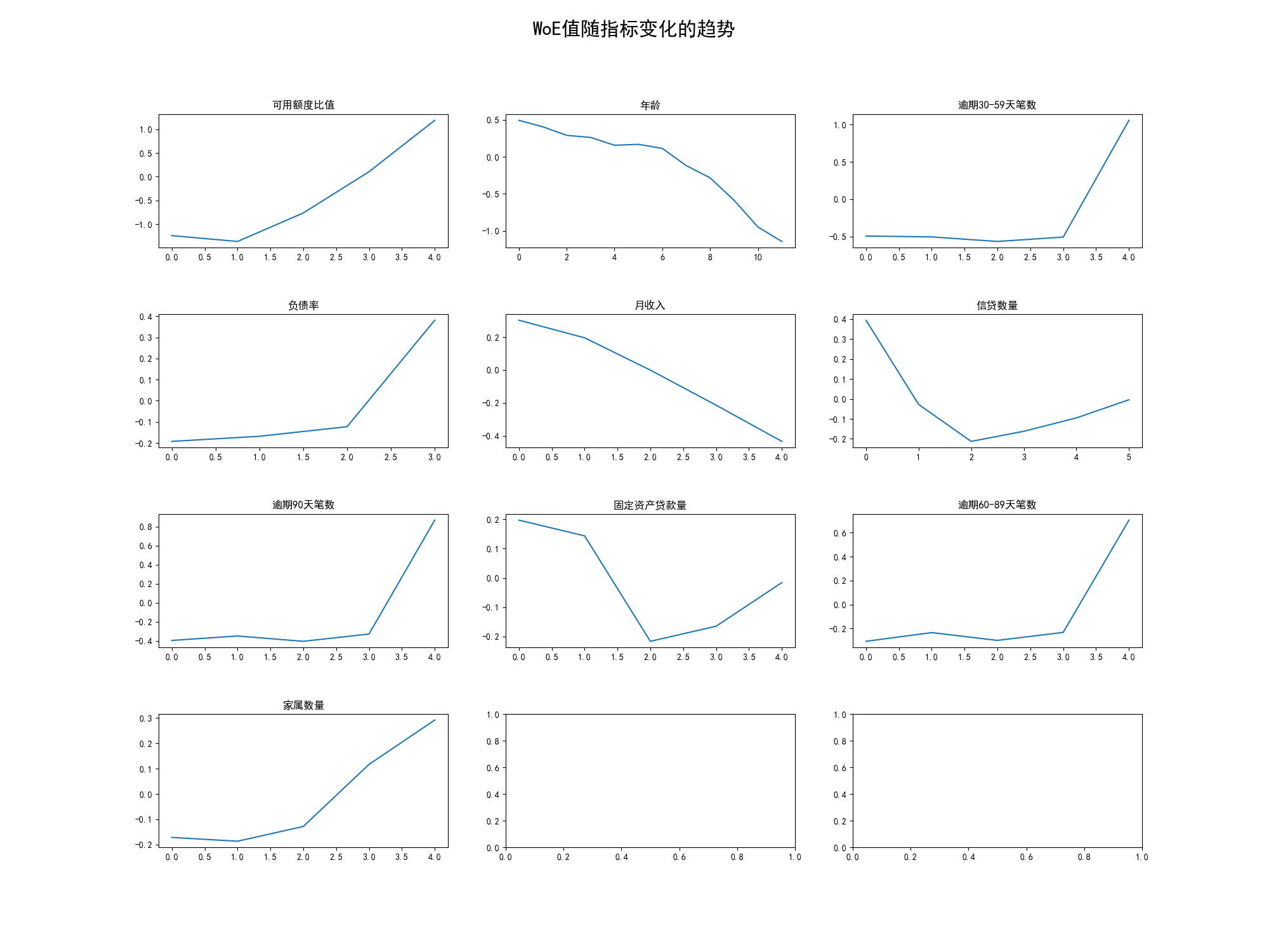
上图为各指标与woe值的关系变化图,大部分都呈现单调变化,而固定资产贷款量和信贷数量大致呈先U型。

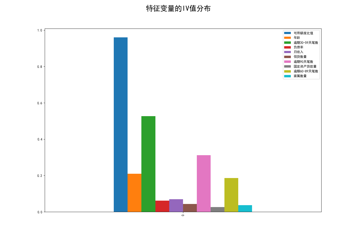
根据前文,已经算出了各变量不同分组对应的IV值,现在利用上述公式计算自变量的IV值。
画出特征变量的IV值分布
ivx1 = x1.iv.sum()
ivx2 = x2.iv.sum()
ivx3 = x3.iv.sum()
ivx4 = x4.iv.sum()
ivx5 = x5.iv.sum()
ivx6 = x6.iv.sum()
ivx7 = x7.iv.sum()
ivx8 = x8.iv.sum()
ivx9 = x9.iv.sum()
ivx10 = x10.iv.sum()
IV = pd.DataFrame({"可用额度比值": ivx1,
                   "年龄": ivx2,
                   "逾期30-59天笔数": ivx3,
                   "负债率": ivx4,
                   "月收入": ivx5,
                   "信贷数量": ivx6,
                   "逾期90天笔数": ivx7,
                   "固定资产贷款量": ivx8,
                   "逾期60-89天笔数": ivx9,
                   "家属数量": ivx10}, index=[0])

ivplot = IV.plot.bar(figsize=(15, 10))
plt.suptitle("特征变量的IV值分布", fontsize=22)
plt.show()
模型分析
基于Logistic回归的评分卡模型建立过程中,一般要将自变量通过WOE进行转化,证据权重(Weight of Evidence,WOE)转换可以将Logistic回归模型转变为标准评分卡格式。
WOE转化
将各变量数据转化为woe值,即将变量的值替换为对应所在分组的WOE值。
# 应用函数,求出各变量分类情况
cut1 = cutdata(train['RevolvingUtilizationOfUnsecuredLines'], 5)
cut2 = cutdata(train['age'], 12)
cut3 = cutdata(train['NumberOfTime30-59DaysPastDueNotWorse'], 5)
cut4 = cutdata(train['DebtRatio'], 4)
cut5 = cutdata(train['MonthlyIncome'], 5)
cut6 = cutdata(train['NumberOfOpenCreditLinesAndLoans'], 6)
cut7 = cutdata(train['NumberOfTimes90DaysLate'], 5)
cut8 = cutdata(train['NumberRealEstateLoansOrLines'], 5)
cut9 = cutdata(train['NumberOfTime60-89DaysPastDueNotWorse'], 5)
cut10 = cutdata(train['NumberOfDependents'], 5)

# 应用上述函数进行数值替换,cut1,cut2...保存了变量分组,x1,x2..保存了woe、iv等值
train_new = pd.DataFrame()
train_new['SeriousDlqin2yrs'] = train['SeriousDlqin2yrs']
train_new['RevolvingUtilizationOfUnsecuredLines'] = replace_train(cut1, x1.woe)
train_new['age'] = replace_train(cut2, x2.woe)
train_new['NumberOfTime30-59DaysPastDueNotWorse'] = replace_train(cut3, x3.woe)
train_new['DebtRatio'] = replace_train(cut4, x4.woe)
train_new['MonthlyIncome'] = replace_train(cut5, x5.woe)
train_new['NumberOfOpenCreditLinesAndLoans'] = replace_train(cut6, x6.woe)
train_new['NumberOfTimes90DaysLate'] = replace_train(cut7, x7.woe)
train_new['NumberRealEstateLoansOrLines'] = replace_train(cut8, x8.woe)
train_new['NumberOfTime60-89DaysPastDueNotWorse'] = replace_train(cut9, x9.woe)
train_new['NumberOfDependents'] = replace_train(cut10, x10.woe)

# WOE转化
print(train_new.head())
WOE转化后前5条数据,为便于展示,表头使用中文显示且只展示部分列
| 好/坏客户 | 可用额度比值 | 年龄 | 负债比例 | 月收入 | 贷款数量 | 90天逾期次数 | 家属数量 |
|---|---|---|---|---|---|---|---|
| 1 | 1.192062 | 0.155663 | 0.380990 | -0.434074 | -0.016137 | -0.394909 | 116546 |
| 0 | 1.192062 | 0.289068 | -0.192007 | 0.302321 | 460.197091 | -0.394909 | -0.128572 |
| 0 | 0.105504 | 0.289068 | -0.192007 | 0.302321 | 0.197091 | -0.866866 | -0.171754 |
| 0 | -0.766298 | 0.491883 | -0.192007 | 0.195328 | 0.197091 | -0.394909 | -0.171754 |
| 0 | -0.766298 | -1.141820 | -0.122528 | 0.195328 | 0.143390 | -0.394909 | -0.128572 |
训练模型
用sklearn包中的模块进行逻辑回归。
# 导入logistic回归模块
from sklearn.linear_model import LogisticRegression
# 导入数据切分函数
from sklearn.model_selection import train_test_split

train_new1 = train_new.drop(
    [
        "DebtRatio",
        "MonthlyIncome",
        "NumberOfOpenCreditLinesAndLoans",
        "NumberRealEstateLoansOrLines",
        "NumberOfDependents"
    ],
    axis=1)
print(train_new1.head())

# 设定自变量
x = train_new1.iloc[:, 1:]
# 设定因变量
y = train_new.iloc[:, 0]

# 将数据集进行切割,分成训练集和测试集,其中样本占比0.8,采用随机抽样
train_x, test_x, train_y, test_y = train_test_split(x, y, train_size=0.8, random_state=4)

# 建立模型
model = LogisticRegression()
# 训练模型,将结果保存为result
result = model.fit(train_x, train_y)
# 预测测试集的y
# pred_y = model.predict(test_x)
# 计算预测精度 正确率
rate = result.score(test_x, test_y)
根据前文的变量选择分析,将负债率、月收入、信贷数量、固定资产贷款量、家属数量变量舍弃,不纳入模型中
| 好/坏客户 | 可用额度比值 | 年龄 | 逾期30-59天笔数 | 逾期90天笔数 | 逾期60-89天笔数 |
|---|---|---|---|---|---|
| 1 | 1.192062 | 0.155663 | 1.058956 | -0.394909 | -0.306393 |
| 0 | 1.192062 | 0.289068 | -0.494457 | -0.394909 | -0.306393 |
| 0 | 0.105504 | 0.289068 | 1.058956 | -0.394909 | -0.306393 |
| 0 | -0.766298 | 0.491883 | -0.494457 | -0.394909 | -0.306393 |
| 0 | -0.766298 | -1.141820 | -0.494457 | -0.394909 | -0.306393 |
模型准确率: 0.9296745725317154
准确率约为0.93,接近于1,初步看来预测效果良好,但是由于所用的样本中坏客户的占比较少,样本不均衡,进一步判断其准确率,评估分类器的分类效果,需要进一步评估模型的效果。
模型效果评估
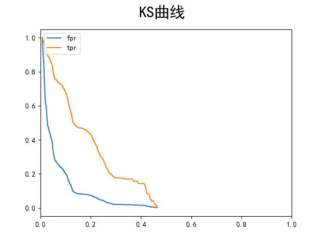
在分类模型评估中,最常用的两种评估标准是K-S值和AUC值,AUC值可以在样本不均衡的情况下准确评估模型的好坏,而K-S值不仅能够评估预测的准确与否,还能度量模型对好坏客户是否有足够的区分度。
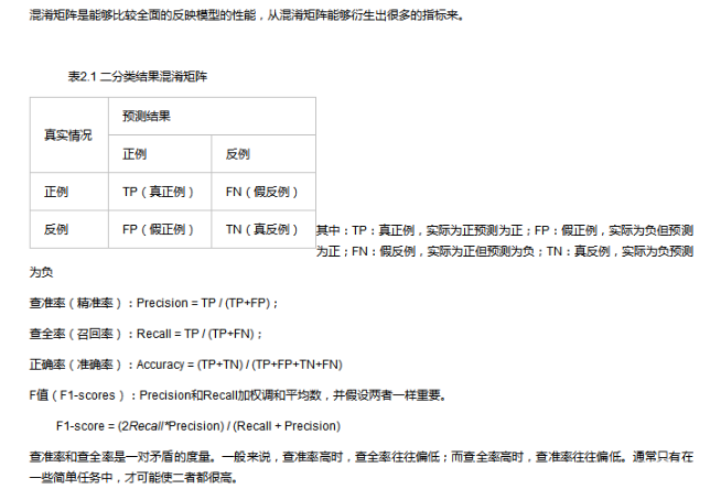
AUC(Area Under the ROC Curve)指标是在二分类问题中,模型评估阶段常被用作最重要的评估指标来衡量模型的稳定性。
根据混淆矩阵,我们可以得到另外两个指标:
真正例率,True Positive Rate:TPR = TP/ (TP+FN)
假正例率, False Postive Rate:FPR = FP/(TN+FP)
另外,真正率是正确预测到的正例数与实际正例数的比值,所以又称为灵敏度(敏感性,sensitive);
对应于灵敏度有一个特异度(特效性,specificity)是正确预测到的负例数与实际负例数的比值(NPV = TN / (TN+FN))。
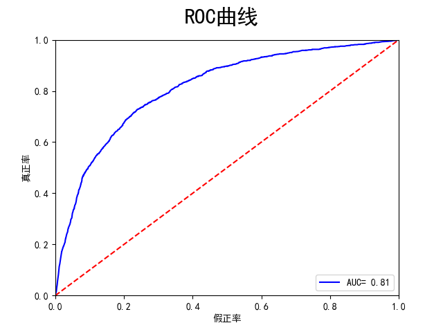
我们以真正例率(TPR)作为纵轴,以假正例率(FPR)作为横轴作图,便得到了ROC曲线,而AUC则是ROC曲线下的面积。AUC的取值为[0.5-1],0.5对应于对角线的“随机猜测模型”。
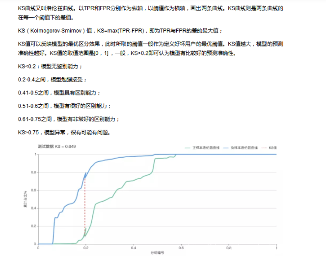
根据模型ks指标画出ks曲线和ROC曲线
# 利用sklearn.metrics计算ROC和AUC值
from sklearn.metrics import roc_curve, auc
# 预测概率predict_proba
proba_y = model.predict_proba(test_x)
# 计算threshold阈值,tpr真正例率,fpr假正例率,大于阈值的视为1即坏客户
fpr, tpr, threshold = roc_curve(test_y, proba_y[:, 1])
# 计算AUC值
roc_auc = auc(fpr, tpr)

# 生成roc曲线
plt.plot(fpr, tpr, 'b', label='AUC= %0.2f' % roc_auc)
plt.legend(loc='lower right')
plt.plot([0, 1], [0, 1], 'r--')
plt.xlim([0, 1])
plt.ylim([0, 1])
plt.ylabel('真正率')
plt.xlabel('假正率')
plt.suptitle("ROC曲线", fontsize=22)
plt.show()
print("AUC值: ", roc_auc)

dataks = pd.DataFrame({"fpr": fpr, "tpr": tpr, "threshold": threshold})
print(dataks.head())

# 按threshold排序
dataks = dataks.sort_values(["threshold"])

# 根据模型ks指标画出ks曲线
plt.plot(dataks.iloc[:, 2], dataks['fpr'], label='fpr')
plt.plot(dataks.iloc[:, 2], dataks['tpr'], label='tpr')
plt.xlim([0, 1])
plt.legend(loc='upper left')
plt.suptitle("KS曲线", fontsize=22)
plt.show()
AUC值:  0.8113359075130762
ks值:  0.48926444898141197
AUC值为0.81,预测效果良好。
ks值为0.47大于0.4,表明分类器具有区分能力。
# 保存模型
np.save("./models/model", scorecard.export(to_frame=True))
信用评分
根据训练的模型或评分卡,对测试数据进行评分。
评分卡
{
	'RevolvingUtilizationOfUnsecuredLines':
		{
			'[-inf ~ 0.302078573)': 209.82,
			'[0.302078573 ~ 0.748569834)': 122.98,
			'[0.748569834 ~ inf)': 48.69
		},
		'DebtRatio':
			{
				'[-inf ~ 0.02)': 159.15,
				'[0.02 ~ 0.4)': 143.7,
				'[0.4 ~ 0.5)': 129.15,
				'[0.5 ~ 2.0)': 91.87,
				'[2.0 ~ inf)': 148.53
			},
		'NumberOfTimes90DaysLate':
			{
				'[-inf ~ 1)': 159.09,
				'[1 ~ inf)': -15.97
			},
		'NumberRealEstateLoansOrLines':
			{
				'[-inf ~ 1)': 123.94,
				'[1 ~ inf)': 140.87
			},
		'NumberOfDependents':
			{
				'[-inf ~ 1.0)': 140.69,
				'[1.0 ~ 3.0)': 126.96,
				'[3.0 ~ inf)': 116.94
			}
		}
}
# 信用卡评分模型测试
def card_model_test():
    card_load = np.load('./models/model.npy', allow_pickle=True)

    # 格式化评分卡
    scard = pd.DataFrame(card_load, columns=['variable', 'bin', 'points'])
    scard['bin'] = scard['bin'].apply(lambda x: x.replace('~', ','))
    scard['bin'] = scard['bin'].apply(lambda x: x.replace(' ', ''))

    scard.info()
    print("card\n", scard.head())

    test_data = pd.read_csv('./data/cs-test.csv')

    # 评分
    score = sc.scorecard_ply(test_data, scard, only_total_score=False)
    print("评分结果\n", score)
完整代码
上面是通过numpy和pandas对数据集进行模型训练的过程。以下是通过toad模型对信用评分模型建模的完整代码
import numpy as np
import pandas as pd
import traceback

from sklearn.linear_model import LogisticRegression
from sklearn.model_selection import train_test_split
from sklearn.metrics import roc_auc_score,roc_curve,auc
import xgboost as xgb

import toad as td
from toad.plot import badrate_plot, proportion_plot, bin_plot
from toad.metrics import KS, F1, AUC

import matplotlib.pyplot as plt
import matplotlib

# 信用评分卡模型训练
class Card_Train:
    def __init__(self):
        super(Card_Train, self).__init__()
        self.sampleFile = './data/cs-training2.csv'
        # 设置matplotlib正常显示中文和负号
        matplotlib.rcParams['font.sans-serif'] = ['SimHei']
        matplotlib.rcParams['axes.unicode_minus'] = False

        # 显示所有列
        pd.set_option('display.max_columns', None)
        # 显示所有行
        pd.set_option('display.max_rows', 10)
        # 设置value的显示长度
        pd.set_option('max_colwidth', 100)
        # 设置1000列时才换行
        pd.set_option('display.width', 1000)

    def output(self, title, data=None, line=False):
        print('\n' + title)

        if line:
            print('-'*100)

        if data is not None:
            print(data)

    def saveFig(self, title):
        plt.suptitle(title, fontsize=22)
        plt.savefig(f'./models/images/{title}.png')
        plt.show()

    def train(self, splitVariable = 'SeriousDlqin2yrs' ):
        # 加载样式数据
        try:
            data = pd.read_csv(self.sampleFile)
        except Exception:
            print("样本文件加载失败", traceback.format_exc())
            return

        # 输出样本数据的相关信息概览
        self.output("样本数据的相关信息概览", line=True)
        data.info()

        # 对变量进行描述性统计分析
        self.output('数据统计分析', data.describe(), True)

        # 输出样本数据前5条信息
        self.output('样本前5条数据', data.head(), True)

        # 样本分区
        Xtr, Xts, Ytr, Yts = train_test_split(data.drop(splitVariable, axis=1),
                                              data[splitVariable],
                                              test_size=0.25,
                                              random_state=450)
        data_tr = pd.concat([Xtr, Ytr], axis=1)
        data_tr['type'] = 'train'
        data_ts = pd.concat([Xts, Yts], axis=1)
        data_ts['type'] = 'test'

        # 保存数据EDA报告
        td.detector.detect(data_tr).to_excel(r'./data/数据EDA结果.xlsx')
        self.output('EDA', td.detector.detect(data_tr), True)

        # 数据特征分析计算特征IV、gini、entropy、unique
        quality = td.quality(data, splitVariable)
        self.output('样本数据特征分析前5条数据', quality.head(), True)

        # 特征预筛选
        selected_train, drop_lst = td.selection.select(data_tr, target=splitVariable,
                                                         empty=0.5,
                                                         corr=0.7,
                                                         return_drop=True,
                                                         exclude='type')
        selected_test = data_ts[selected_train.columns]

        # 特征分箱
        combiner = td.transform.Combiner()

        # 训练数据并制定分箱方法,需要分箱的变量共7个
        combiner.fit(selected_train,
                     y=splitVariable,
                     method='chi',
                     min_samples=0.05,
                     exclude='type')

        # 以字典的形式保存分箱结果
        bins = combiner.export()
        self.output('特征分箱结果', bins, True)

        # 查看每个特征的分箱结果
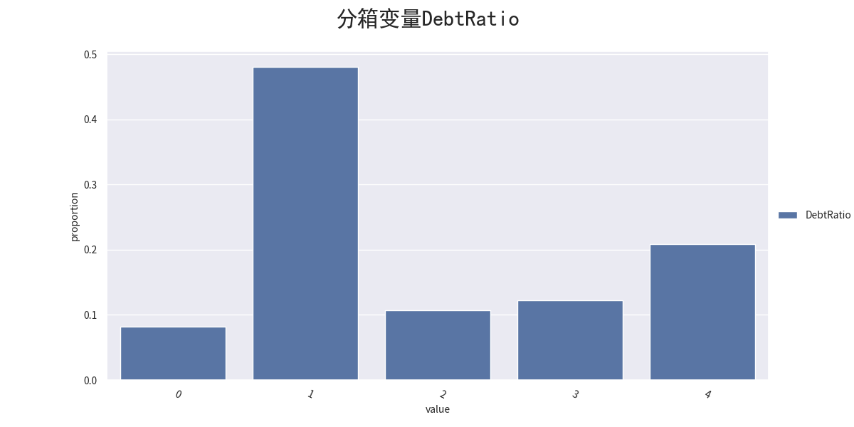
        self.output('DebtRatio分箱cut:', bins['DebtRatio'])
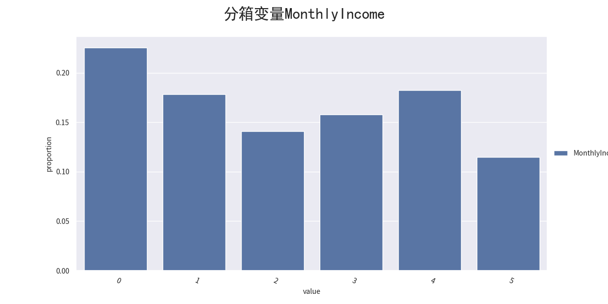
        self.output('MonthlyIncome分箱cut', bins['MonthlyIncome'])
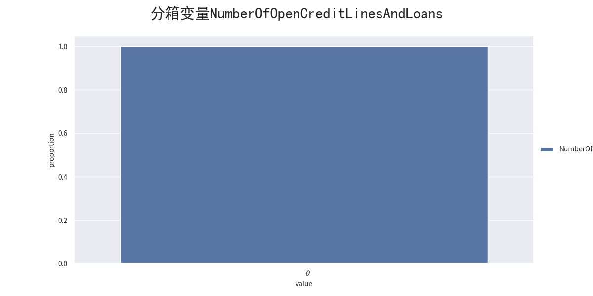
        self.output('NumberOfOpenCreditLinesAndLoans分箱cut',
                    bins['NumberOfOpenCreditLinesAndLoans'])
        self.output('NumberRealEstateLoansOrLines分箱cut',
                    bins['NumberRealEstateLoansOrLines'])
        self.output('NumberOfTimes90DaysLate分箱cut', bins['NumberOfTimes90DaysLate'])
        self.output('RevolvingUtilizationOfUnsecuredLines分箱cut',
                    bins['RevolvingUtilizationOfUnsecuredLines'])
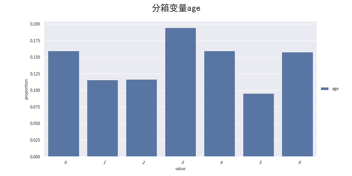
        self.output('age分箱cut', bins['age'])

        # 使用combine.transform()方法对数据进行分箱转换
        selected_train_bin = combiner.transform(selected_train)

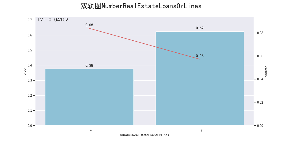
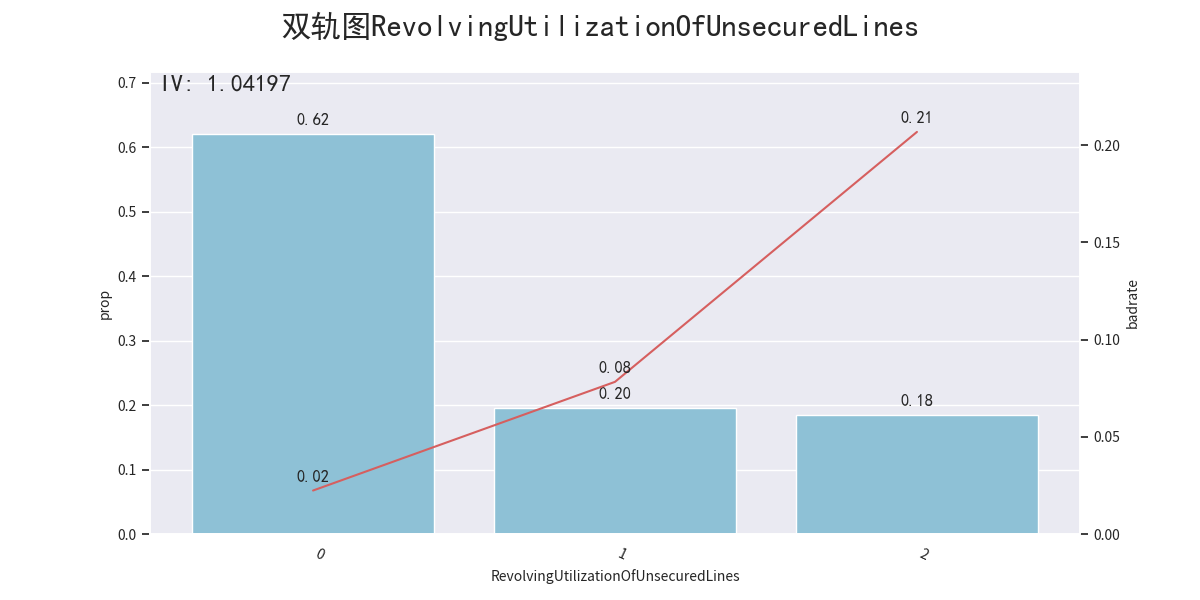
        # 画分箱图,使用bin_plot函数绘制双轨图和分箱占比、分箱坏账率关系图
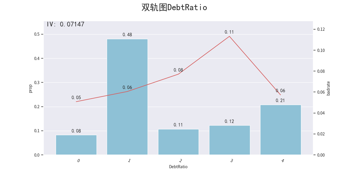
        proportion_plot(selected_train_bin['DebtRatio'])
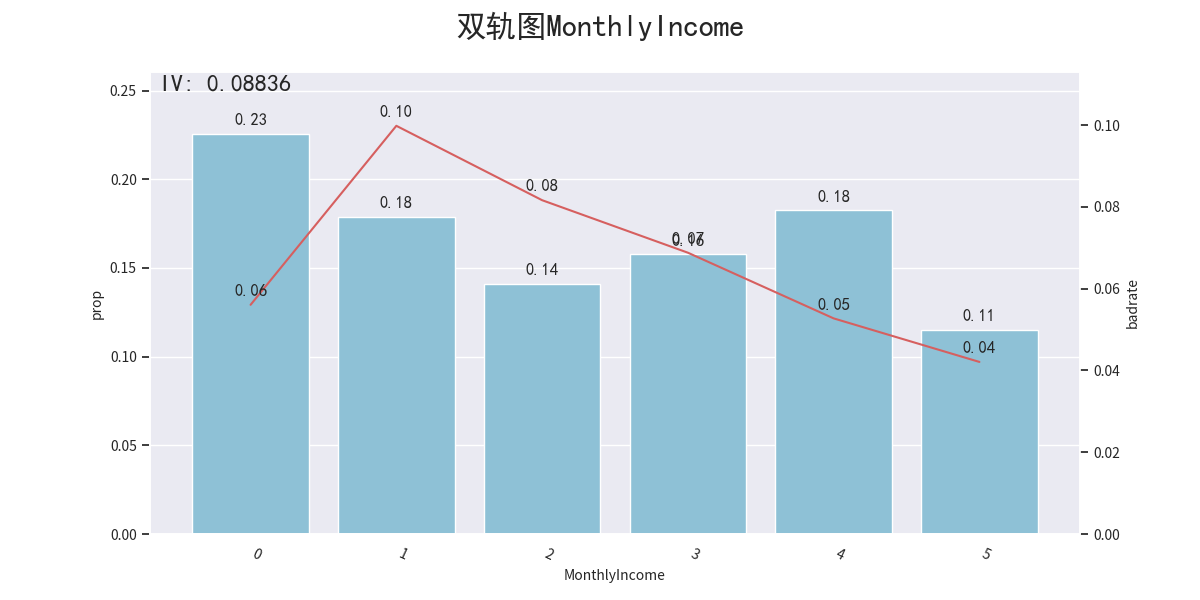
        proportion_plot(selected_train_bin['MonthlyIncome'])
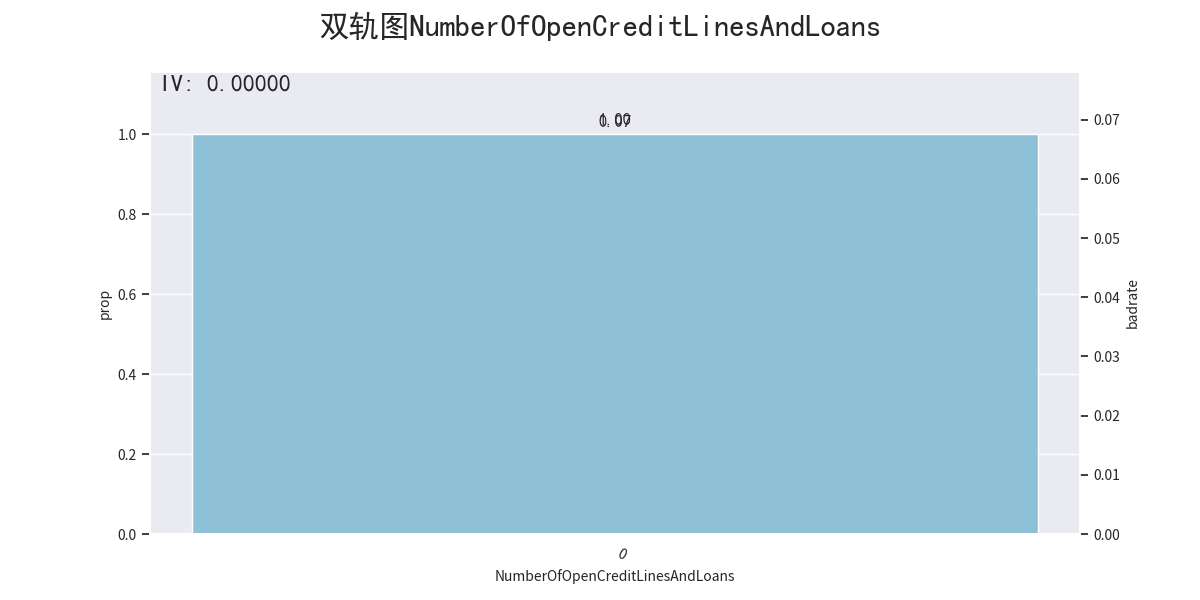
        proportion_plot(selected_train_bin['NumberOfOpenCreditLinesAndLoans'])
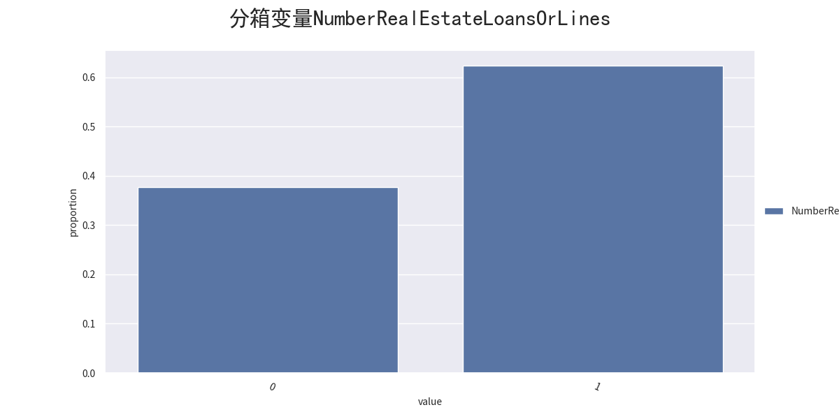
        proportion_plot(selected_train_bin['NumberRealEstateLoansOrLines'])
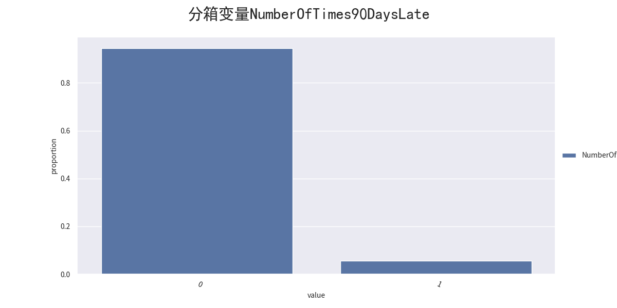
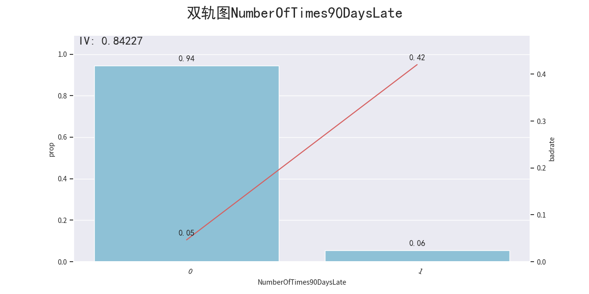
        proportion_plot(selected_train_bin['NumberOfTimes90DaysLate'])
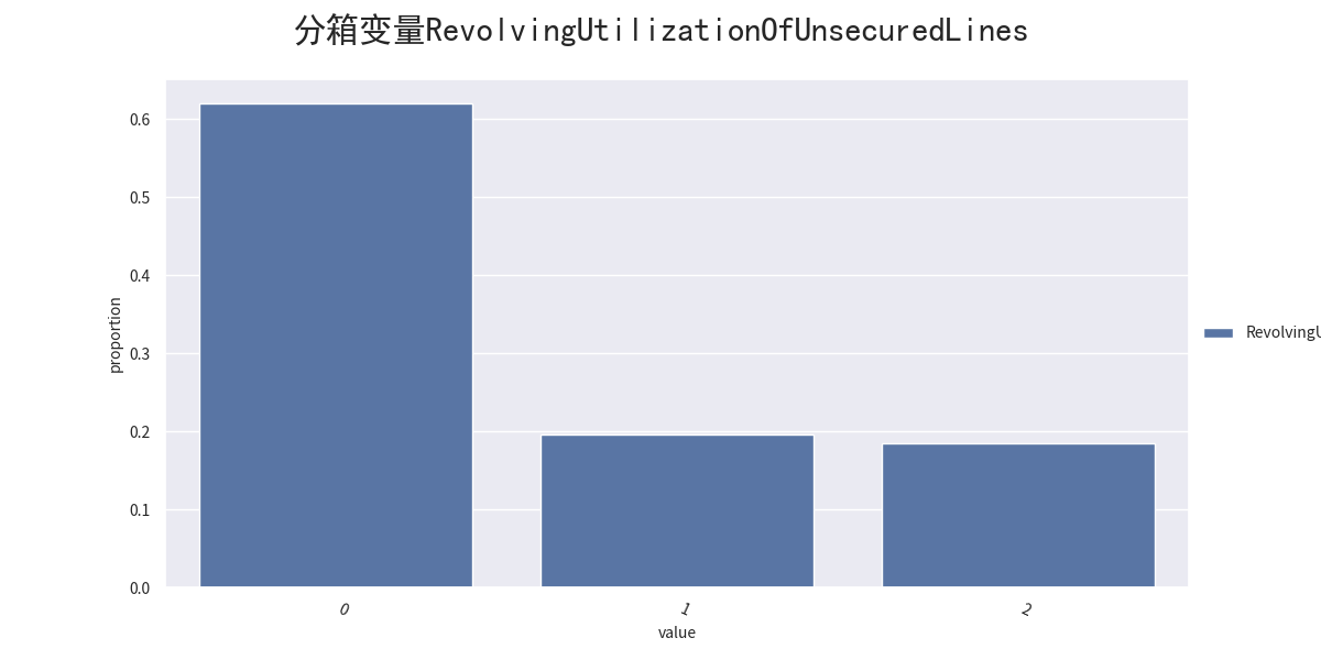
        proportion_plot(selected_train_bin['RevolvingUtilizationOfUnsecuredLines'])
        proportion_plot(selected_train_bin['age'])

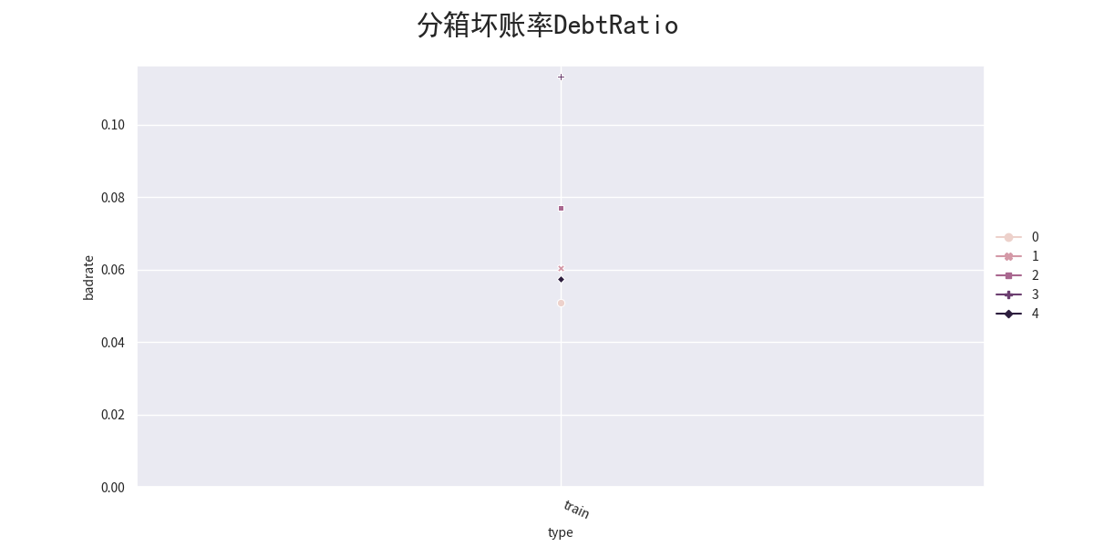
        badrate_plot(selected_train_bin, target=splitVariable, x='type', by='DebtRatio')
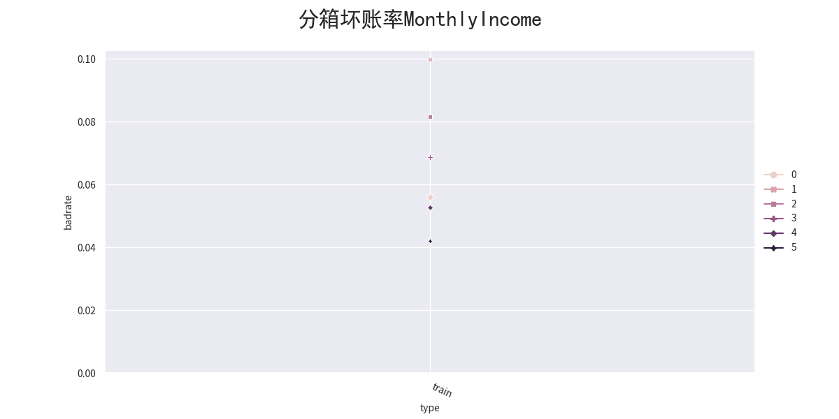
        badrate_plot(selected_train_bin, target=splitVariable, x='type',
                     by='MonthlyIncome')
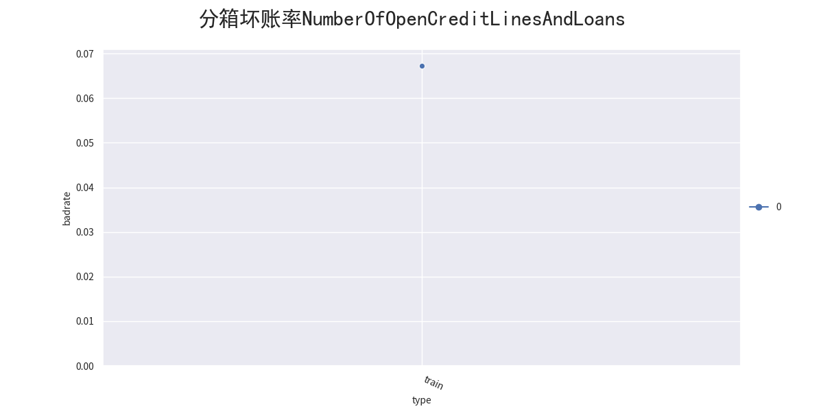
        badrate_plot(selected_train_bin, target=splitVariable, x='type',
                     by='NumberOfOpenCreditLinesAndLoans')
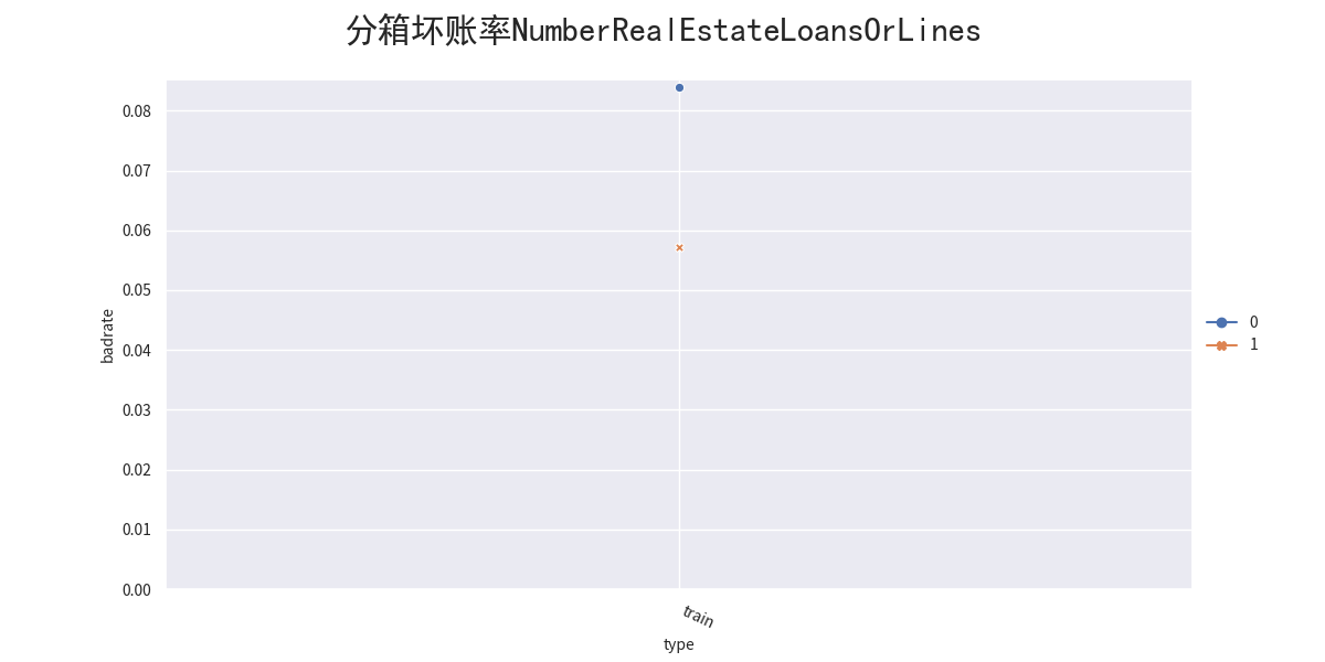
        badrate_plot(selected_train_bin, target=splitVariable, x='type',
                     by='NumberRealEstateLoansOrLines')
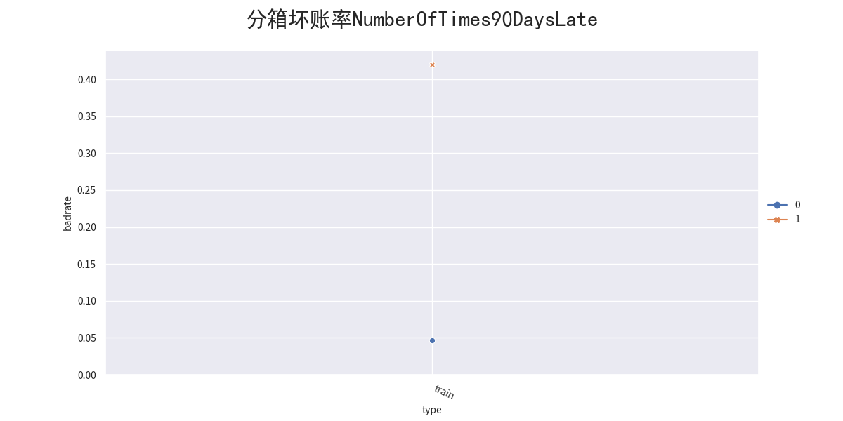
        badrate_plot(selected_train_bin, target=splitVariable, x='type',
                     by='NumberOfTimes90DaysLate')
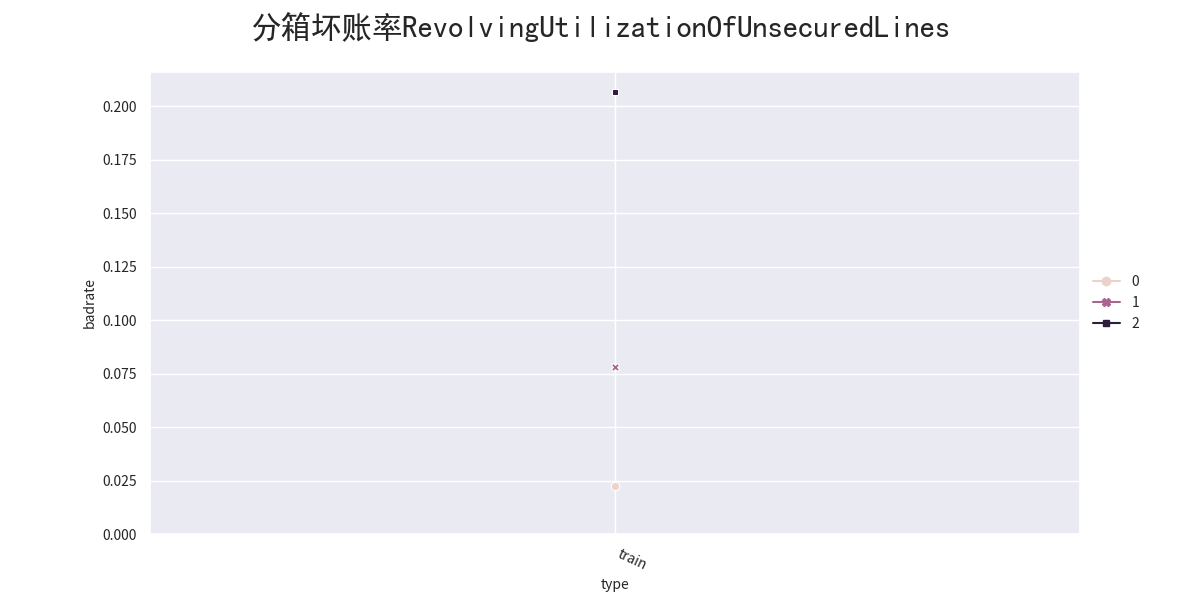
        badrate_plot(selected_train_bin, target=splitVariable, x='type',
                     by='RevolvingUtilizationOfUnsecuredLines')
        badrate_plot(selected_train_bin, target=splitVariable, x='type', by='age')

        bin_plot(selected_train_bin, x='DebtRatio', target=splitVariable)
        bin_plot(selected_train_bin, x='MonthlyIncome', target=splitVariable)
        bin_plot(selected_train_bin, x='NumberOfOpenCreditLinesAndLoans',
                 target=splitVariable)
        bin_plot(selected_train_bin, x='NumberRealEstateLoansOrLines',
                 target=splitVariable)
        bin_plot(selected_train_bin, x='NumberOfTimes90DaysLate', target=splitVariable)
        bin_plot(selected_train_bin, x='RevolvingUtilizationOfUnsecuredLines',
                 target=splitVariable)
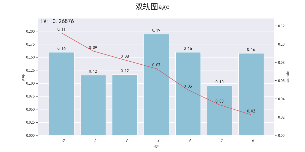
        bin_plot(selected_train_bin, x='age', target=splitVariable)

        # 调整合并分箱 定义调整分箱 调整分箱切分点
        bins_adj = bins
        bins_adj["age"] = [22, 35, 45, 60]
        bins_adj["NumberOfOpenCreditLinesAndLoans"] = [2]
        bins_adj["DebtRatio"] = [0.02, 0.4, 0.5, 2]

        # 定义分类合并器
        combiner2 = td.transform.Combiner()  # 定义分箱combiner
        combiner2.set_rules(bins_adj)        # 设置需要施加的分箱

        # 应用调整分箱
        selected_train_binadj = combiner2.transform(selected_train)

        # 画分箱坏账率图
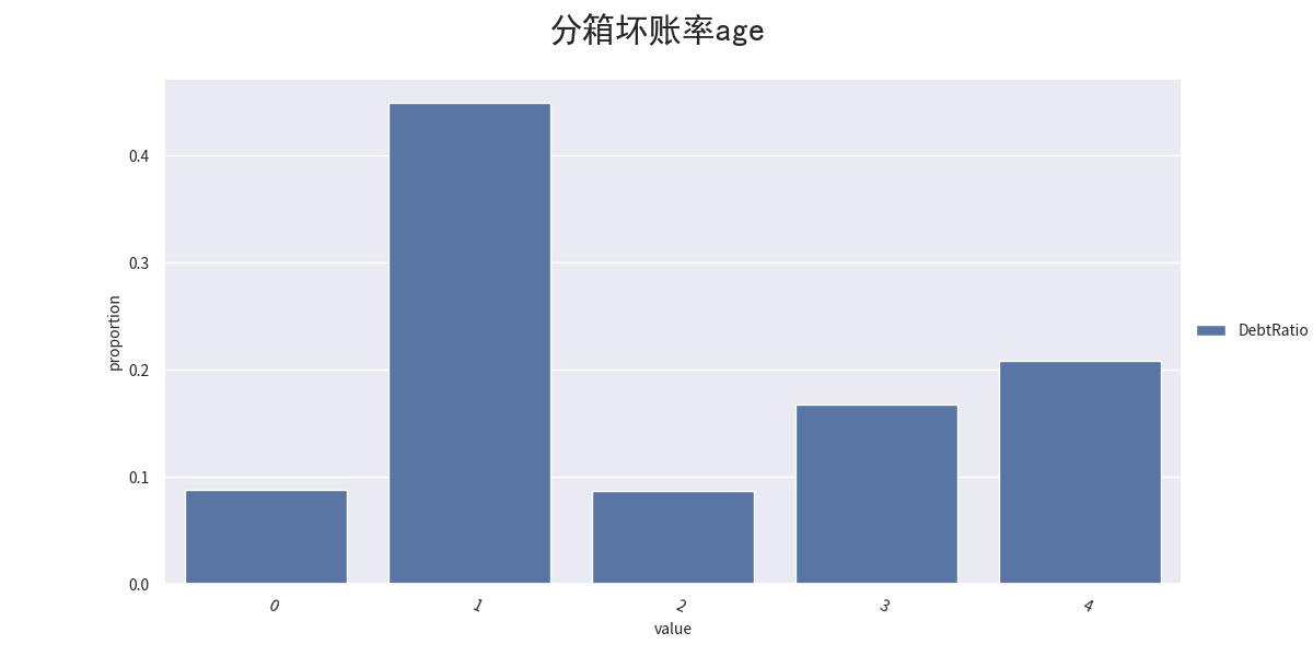
        proportion_plot(selected_train_binadj['DebtRatio'])
        self.saveFig('分箱坏账率age')
        proportion_plot(selected_train_binadj['MonthlyIncome'])
        proportion_plot(selected_train_binadj['NumberOfOpenCreditLinesAndLoans'])
        proportion_plot(selected_train_binadj['NumberRealEstateLoansOrLines'])
        proportion_plot(selected_train_binadj['NumberOfTimes90DaysLate'])
        proportion_plot(selected_train_binadj['RevolvingUtilizationOfUnsecuredLines'])
        proportion_plot(selected_train_binadj['age'])

        badrate_plot(selected_train_binadj, target=splitVariable, x='type',
                     by='DebtRatio')
        badrate_plot(selected_train_binadj, target=splitVariable, x='type',
                     by='MonthlyIncome')
        badrate_plot(selected_train_binadj, target=splitVariable, x='type',
                     by='NumberOfOpenCreditLinesAndLoans')
        badrate_plot(selected_train_binadj, target=splitVariable, x='type',
                     by='NumberRealEstateLoansOrLines')
        badrate_plot(selected_train_binadj, target=splitVariable, x='type',
                     by='NumberOfTimes90DaysLate')
        badrate_plot(selected_train_binadj, target=splitVariable, x='type',
                     by='RevolvingUtilizationOfUnsecuredLines')
        badrate_plot(selected_train_binadj, target=splitVariable, x='type', by='age')
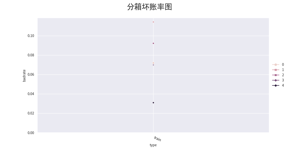
        plt.suptitle("分箱坏账率图", fontsize=22)
        plt.show()

        self.output('WOE值', line=True)
        # 转换WOE值
        combiner.set_rules(bins_adj)

        # 特征转化的值转化为分箱的箱号
        selected_train_binadj = combiner.transform(selected_train)
        selected_test_binadj = combiner.transform(selected_test)

        # 定义WOE转换器
        WOETransformer = td.transform.WOETransformer()

        # 对WOE的值进行转化,映射到原数据集上,对训练集使用fit_transform()方法转化,
        # 对测试集使用transform()方法转化
        data_tr_woe = WOETransformer.fit_transform(selected_train_binadj,
                                                   selected_train_binadj[splitVariable],
                                                   exclude=[splitVariable, 'type'])
        data_ts_woe = WOETransformer.transform(selected_test_binadj)

        # 9.特征选择,使用stepwise()方法选择变量
        train_final = td.selection.stepwise(data_tr_woe.drop('type', axis=1),
                                              target=splitVariable,
                                              direction='both',
                                              criterion='aic'
                                              )
        test_final = data_ts_woe[train_final.columns]
        self.output('特征选择', train_final.shape)

        # 模型训练
        self.output('模型训练', line=True)
        # 准备数据
        Xtr = train_final.drop(splitVariable, axis=1)
        Ytr = train_final[splitVariable]

        # 逻辑回归模型拟合
        lr = LogisticRegression()
        lr.fit(Xtr, Ytr)

        # 打印模型拟合的参数
        self.output('模型拟合参数coef_', lr.coef_)
        self.output('模型拟合参数intercept_', lr.intercept_)

        # 模型评估
        self.output('模型评估', line=True)
        # 评估在训练集上的模型表现
        EYtr_proba = lr.predict_proba(Xtr)[:, 1]
        EYtr_proba = lr.predict(Xtr)

        self.output('train F1:', F1(EYtr_proba, Ytr))
        self.output('train KS:', KS(EYtr_proba, Ytr))
        self.output('train AUC:', AUC(EYtr_proba, Ytr))

        # 分值排序性
        tr_bucket = td.metrics.KS_bucket(EYtr_proba, Ytr, bucket=10, method='quantile')

        # 等频分段
        self.output('等频分段', tr_bucket)

        # 模型验证
        self.output('模型验证', line=True)
        # 在测试集上的模型表现
        Xts = test_final.drop('SeriousDlqin2yrs', axis=1)
        Yts = test_final['SeriousDlqin2yrs']

        EYtr_proba = lr.predict_proba(Xts)[:, 1]
        # EYts = lr.predict(Xts)

        self.output('train F1:', F1(EYtr_proba, Yts))
        self.output('train KS:', KS(EYtr_proba, Yts))
        self.output('train AUC:', AUC(EYtr_proba, Yts))

        # 基于分箱之后的数据,比较训练集、测试集变量稳定性分布是否有显著差异
        psi = td.metrics.PSI(train_final, test_final).sort_values(0)
        psi = psi.reset_index()
        psi = psi.rename(columns={'index':'feature', 0:'psi'})
        self.output('PSI:', psi, line=True)
        self.output('AUC:', AUC(EYtr_proba, Yts))

        # 分值转换
        self.output('分值转换', line=True)
        scorecard = td.ScoreCard(combiner=combiner, transer=WOETransformer, C=0.1)
        scorecard.fit(Xtr, Ytr)
        # 保存模型
        np.save("./models/model", scorecard.export(to_frame=True))
        self.output("保存模型 model.npy")

        score = scorecard.predict(data)
        self.output("测试数据评分", score)

        self.output('评分卡', scorecard.export())

    # LR 模型训练
    def lr_model(self, x, y, valx, valy, offx, offy, c):
        model = LogisticRegression(C=c, class_weight='balanced')
        model.fit(x, y)

        # dev
        y_pred = model.predict_proba(x)[:, 1]
        fpr_dev, tpr_dev, _ = roc_curve(y, y_pred)
        dev_ks = abs(fpr_dev - tpr_dev).max()
        print('dev_ks:', dev_ks)

        y_pred = model.predict_proba(valx)[:, 1]
        fpr_val, tpr_val, _ = roc_curve(valy, y_pred)
        val_ks = abs(fpr_val - tpr_val).max()
        print('val_ks:', val_ks)

        y_pred = model.predict_proba(offx)[:, 1]
        fpr_off, tpr_off, _ = roc_curve(offy, y_pred)
        off_ks = abs(fpr_off - tpr_off).max()
        print('off_ks:', off_ks)

        plt.plot(fpr_dev, tpr_dev, label='dev')
        plt.plot(fpr_val, tpr_val, label='val')
        plt.plot(fpr_off, tpr_off, label='off')
        plt.plot([0, 1], [0, 1], 'k--')
        plt.xlabel('假阳性率')
        plt.ylabel('真阳性率')
        plt.legend(loc='best')
        plt.suptitle('LR模型ROC曲线', fontsize=22)
        plt.show()


    # XGB 模型训练
    def xgb_model(self, x, y, valx, valy, offx, offy):
        model = xgb.XGBClassifier(learning_rate=0.05,
                                  n_estimators=400,
                                  max_depth=2,
                                  min_child_weight=1,
                                  subsample=1,
                                  nthread=-1,
                                  scale_pos_weight=1,
                                  random_state=1,
                                  n_jobs=-1,
                                  reg_lambda=300)
        model.fit(x, y)

        # dev
        y_pred = model.predict_proba(x)[:, 1]
        fpr_dev, tpr_dev, _ = roc_curve(y, y_pred)
        dev_ks = abs(fpr_dev - tpr_dev).max()
        print('dev_ks:', dev_ks)

        y_pred = model.predict_proba(valx)[:, 1]
        fpr_val, tpr_val, _ = roc_curve(valy, y_pred)
        val_ks = abs(fpr_val - tpr_val).max()
        print('val_ks:', val_ks)

        y_pred = model.predict_proba(offx)[:, 1]
        fpr_off, tpr_off, _ = roc_curve(offy, y_pred)
        off_ks = abs(fpr_off - tpr_off).max()
        print('off_ks:', off_ks)

        plt.plot(fpr_dev, tpr_dev, label='dev')
        plt.plot(fpr_val, tpr_val, label='val')
        plt.plot(fpr_off, tpr_off, label='off')
        plt.plot([0, 1], [0, 1], 'k--')
        plt.xlabel('假阳性率')
        plt.ylabel('真阳性率')
        plt.legend(loc='best')
        plt.suptitle('XGB模型ROC曲线', fontsize=22)
        plt.savefig('./models/images/XGB模型ROC曲线.png')
        plt.show()
图形结果输出